In Part 1, we explored the mathematical foundations of convolutions. In Part 2, we built custom Conv2D layers, pooling operations, and complete CNN architectures in pure PyTorch.
Now, we reap the rewards: training our CNN on MNIST and peering inside the black box. After training, we can visualize what features the learned filters actually detect and analyze how feature maps represent information at different depths of the network.
Training Results
Our SimpleCNN achieves strong performance on MNIST digit classification:
- Training accuracy: ~99%
- Test accuracy: ~99%
- Convergence: Within 10 epochs
The training curves show characteristic CNN behavior: rapid initial learning followed by gradual refinement as the network fine-tunes its feature detectors.
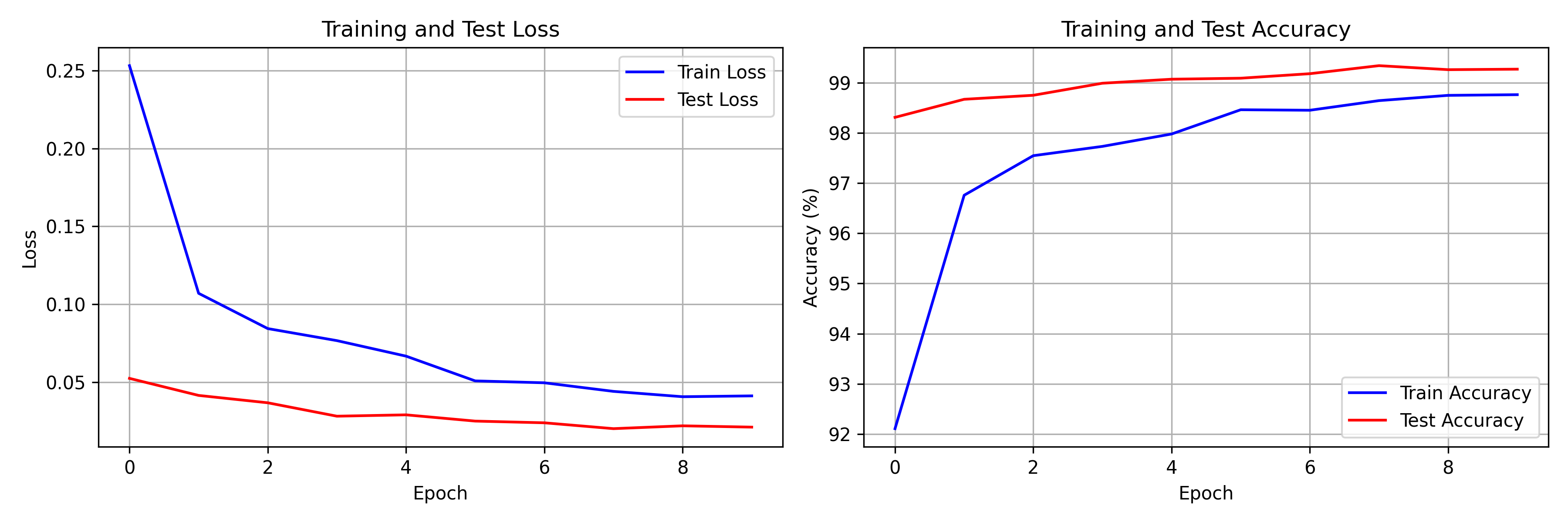
Training and test loss/accuracy curves over 10 epochs. The CNN converges quickly, with both train and test metrics closely tracking — indicating good generalization with no significant overfitting thanks to dropout regularization.
Visualizing Learned Filters
First Layer Filters
The first convolutional layer learns interpretable, low-level features:
- Edge detectors (vertical, horizontal, diagonal orientations)
- Blob detectors responding to local intensity patterns
- Simple texture patterns capturing fine-grained structure
These match findings from neuroscience: early visual cortex neurons also respond to oriented edges and simple spatial frequency patterns.
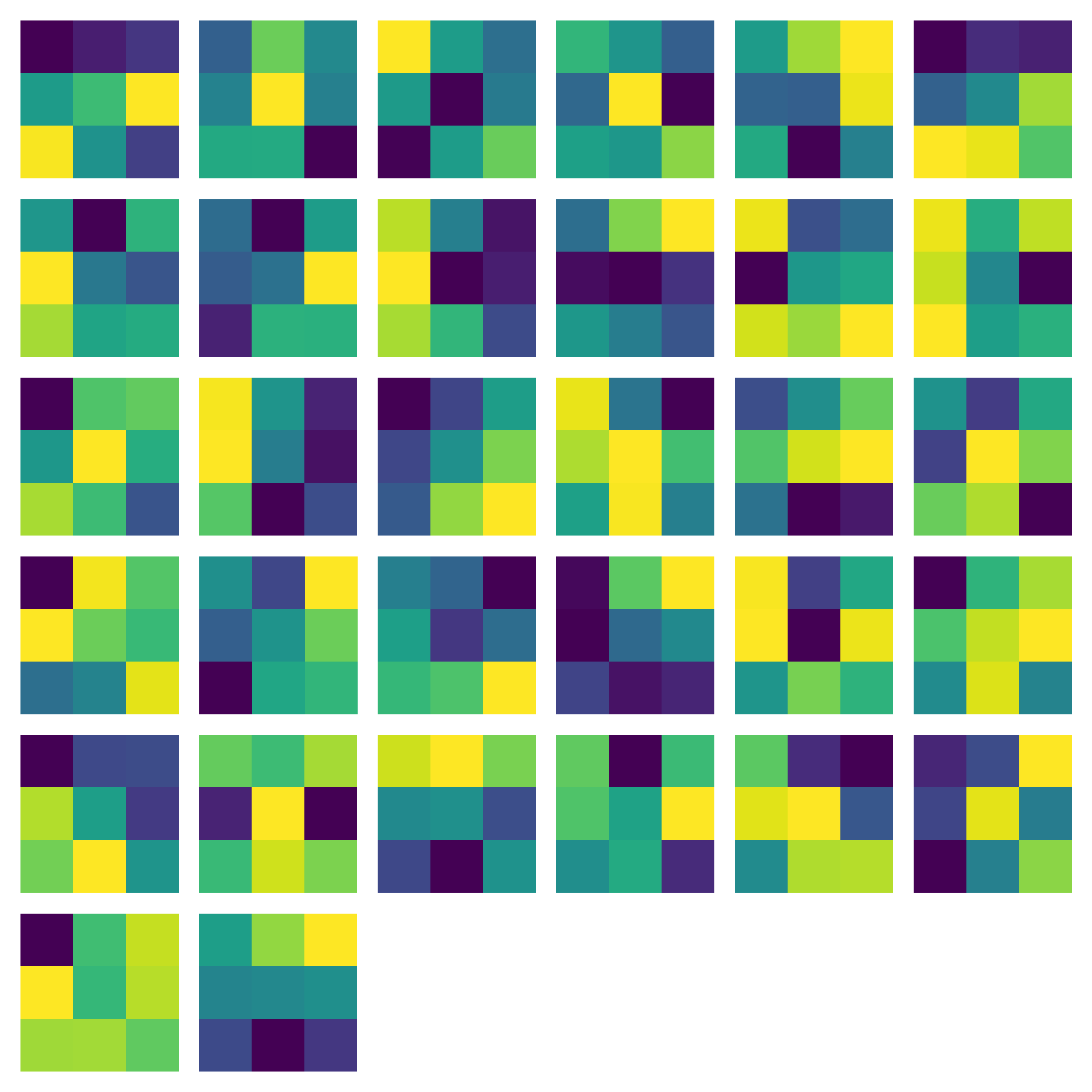
The 32 learned convolutional filters from the first layer of our SimpleCNN. Each 3x3 filter has learned to detect a specific low-level feature. We normalize each filter to $[0, 1]$ for visualization. Notice the variety of edge orientations and blob patterns the network has discovered autonomously through backpropagation.
Feature Map Analysis
What Are Feature Maps?
Feature maps are the activations produced when an input image passes through a convolutional layer. Each map represents the spatial presence of a specific feature — bright regions indicate where the corresponding filter responds strongly to the input.
Progressive Abstraction
As we move deeper through the network, the feature maps show progressive abstraction:
- Layer 1: Responds to edges and simple patterns in the raw image
- Layer 2: Combines edges into shapes, contours, and motifs
- Deeper layers: Detect complex patterns and discriminative digit features
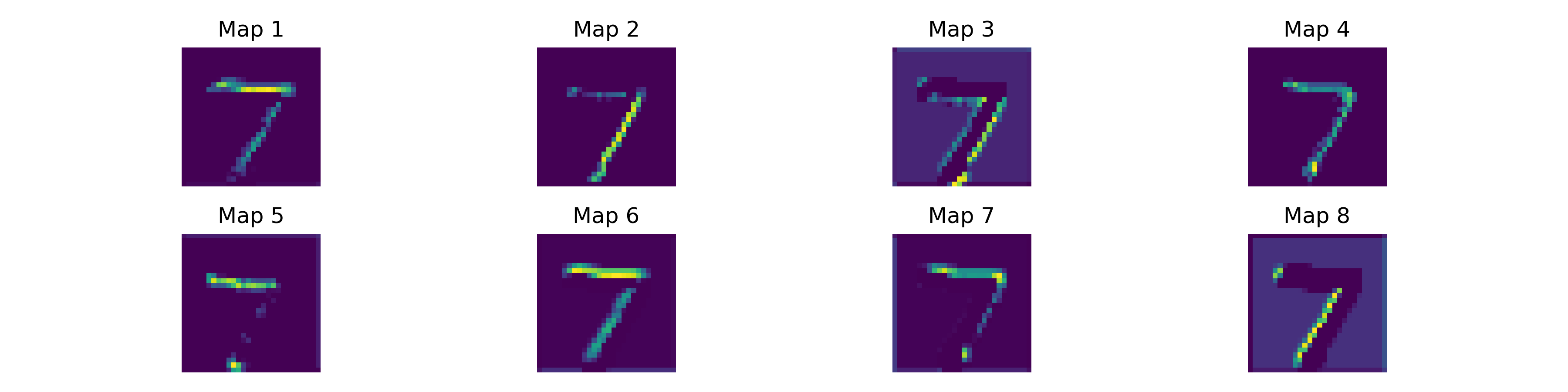
Feature map activations from the first convolutional layer for a sample MNIST digit. Each map highlights different structural aspects of the input — some respond to horizontal strokes, others to vertical edges or curves. The ReLU activation creates sparse maps where most neurons are inactive, focusing the representation on the most salient features.
Sparse Activations
ReLU creates sparse feature maps — most neurons are inactive (zero) for any given input. This sparsity is computationally efficient and may aid generalization by encouraging the network to develop more robust, non-redundant feature detectors.
Why CNNs Work
Inductive Biases
CNNs encode powerful assumptions about visual data that make them remarkably effective:
- Locality: Nearby pixels are correlated — features are local
- Translation equivariance: Features are location-independent
- Compositionality: Complex patterns are built from simpler ones
Comparison to Fully Connected Networks
For image tasks, CNNs vastly outperform fully connected networks because of:
- Parameter efficiency: Weight sharing reduces parameters by orders of magnitude
- Spatial structure preservation: The 2D structure of images is maintained
- Hierarchical feature learning: Layer-by-layer composition of increasingly abstract representations
Conclusion
CNNs remain foundational to computer vision. While Vision Transformers have gained popularity for large-scale tasks, CNNs offer unmatched efficiency, interpretability, and strong inductive biases for visual data. Understanding CNNs is essential for any deep learning practitioner.
We built this entirely from scratch in PyTorch — no pre-built convolutional layers, no pre-trained weights. By seeing the raw filters learn edge detectors and watching feature maps light up with hierarchical abstractions, we demystify the core architecture that launched the deep learning revolution.
Thank you for following this 3-part "Build in Public" series on Convolutional Neural Networks. Stay connected on LinkedIn for future architectural tear-downs!