Deconstructing CNNs from Scratch

Training Setup

The SimpleCNN architecture follows the classic Conv-ReLU-Pool pattern: two convolutional blocks (32 and 64 filters, both 3x3 with padding) each followed by 2x2 max pooling, then two fully connected layers (3136 to 128, 128 to 10) with 50% dropout between them. We trained with Adam (learning rate 0.001), cross-entropy loss, batch size 64, and a StepLR scheduler that halves the learning rate at epoch 5. All convolution and pooling operations were built from scratch using custom Conv2D and MaxPool2D modules with Xavier weight initialization.

Training Results

SimpleCNN on MNIST, 10 epochs:

• Final training accuracy: 98.76% (loss: 0.0412)
• Best test accuracy: 99.34% at epoch 8 (loss: 0.0202)
• Final test accuracy: 99.27% (loss: 0.0212)

The network hits 98.31% test accuracy after just one epoch -- already strong enough to classify most digits correctly. By epoch 2, test accuracy climbs to 98.67%. It crosses 99% at epoch 5 (99.07%) and peaks at 99.34% in epoch 8. The final two epochs show slight fluctuation (99.26% at epoch 9, 99.27% at epoch 10), characteristic of the learning rate step kicking in and the model settling into a flat region of the loss landscape.

Train and test curves track closely throughout -- the gap between train loss (0.0412) and test loss (0.0212) at convergence actually favors the test set, which indicates dropout is doing its job as a regularizer during training. Total training time was under 5 minutes on CPU, covering all 10 epochs across 60,000 training images.

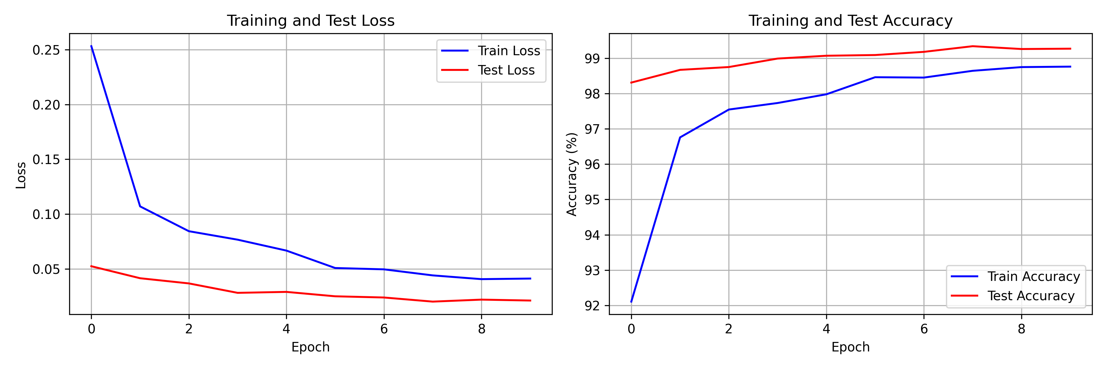
Loss and accuracy over 10 epochs. Train and test metrics stay close, indicating no significant overfitting.

Visualizing Learned Filters

First Layer Filters

The first convolutional layer learns interpretable features:

• Edge detectors (vertical, horizontal, diagonal)
• Blob detectors for local intensity patterns
• Simple texture patterns

This mirrors neuroscience findings — V1 neurons in the visual cortex respond to oriented edges in much the same way.

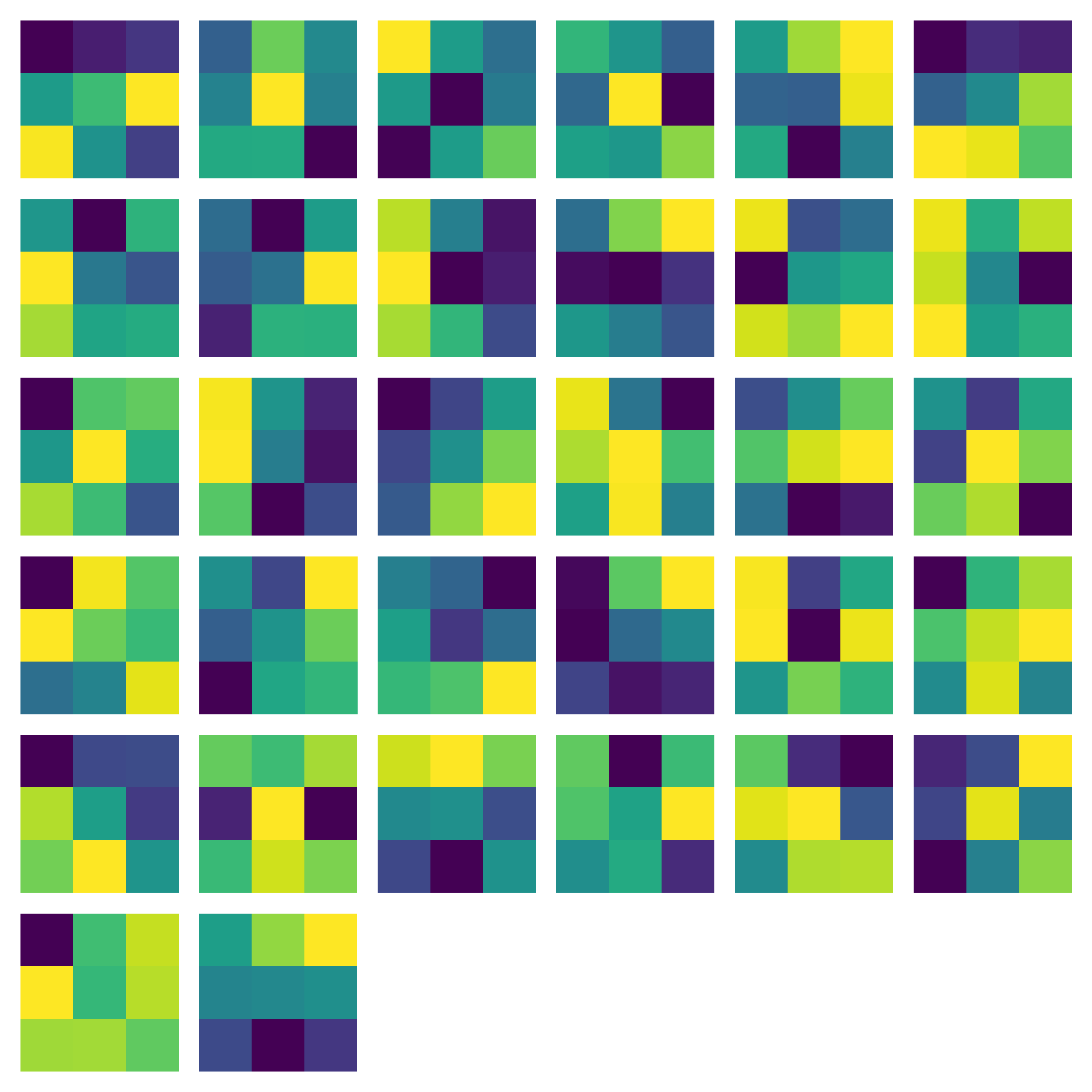
All 32 first-layer filters, normalized to $[0, 1]$ for display. Each 3x3 kernel has specialized to detect a different low-level pattern.

Feature Map Analysis

Progressive Abstraction

Feature maps are the activations produced when an input passes through a convolutional layer. Each map shows where a specific filter fires strongly. Deeper layers combine these into increasingly abstract representations:

• Layer 1: Edges and simple patterns from the raw image
• Layer 2: Edges combined into shapes and contours
• Deeper layers: Discriminative patterns for digit identity

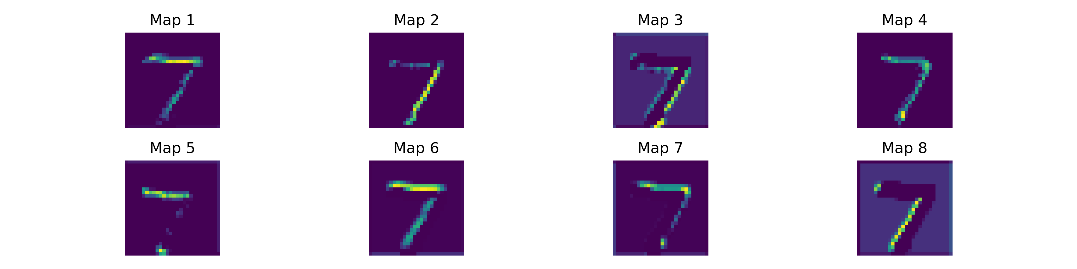
First-layer feature maps for a sample MNIST digit. Different maps respond to horizontal strokes, vertical edges, and curves. ReLU zeroes out most activations, keeping the representation sparse.

Sparse Activations

ReLU produces sparse feature maps -- most neurons output zero for any given input. This sparsity is computationally cheap and likely helps generalization. For a given MNIST digit, only a fraction of the 32 first-layer feature maps activate strongly. A "1" lights up the vertical edge detectors while leaving horizontal and diagonal maps near zero. A "0" activates curved-edge detectors around its contour and suppresses everything else. This selective firing is what allows a compact 421K-parameter network to distinguish ten digit classes with over 99% accuracy.

Why CNNs Work

Inductive Biases

CNNs bake in three assumptions about visual data:

• Locality: Nearby pixels are correlated
• Translation equivariance: Features are location-independent
• Compositionality: Complex patterns build from simpler ones

vs. Fully Connected Networks

For images, CNNs outperform FC networks because of weight sharing (far fewer parameters), spatial structure preservation, and hierarchical feature composition. Consider the numbers: our SimpleCNN uses 421,642 parameters to reach 99.3% on MNIST. A fully connected network processing the same 28x28 images would need $784 \times h$ parameters in its first layer alone. To match the CNN's representational capacity, you would need hidden layers of comparable width -- easily pushing past a million parameters -- and it would still lack translation invariance. Shift a digit a few pixels to the right and the FC network must relearn the pattern; the CNN recognizes it automatically because the same kernel scans every position.

Conclusion

CNNs remain foundational to computer vision. Vision Transformers have taken over at the large-scale end, but CNNs still offer better efficiency and stronger inductive biases when data or compute is limited.

Everything here was built from scratch — no pre-built conv layers, no pre-trained weights. Watching 3x3 kernels independently converge to edge detectors is a good way to build intuition for what these networks are actually doing.