Part 1 covered the math. Part 2 built the UNet and training loop. Now we train and generate.
We trained the DDPM on MNIST for 15 epochs with a 324,705-parameter UNet. Classifying MNIST is trivial; generating it from a 1,000-step Markov chain is a different problem entirely, and it exposes the same mechanics that power large-scale models like DALL-E and Sora.
The Training Process
The objective: predict the Gaussian noise $\epsilon$ added at a random timestep $t$, minimize MSE. Loss dropped from 0.2203 at epoch 1 to 0.0619 at epoch 15 -- a 72% reduction. The sharpest improvement came in the first 3 epochs (0.2203 to 0.0987), with steady gains after that.
Epoch-by-Epoch Breakdown
The training ran on Apple Silicon (MPS backend) with a batch size of 128 and a learning rate of $2 \times 10^{-4}$ using Adam. Here is the full loss trajectory:
- Epochs 1-3 (rapid learning): 0.2203, 0.1124, 0.0987. The loss halved in a single epoch, then dropped another 12%. This is where the network learns the coarse structure -- the broad outlines of digits at high noise levels.
- Epochs 4-6 (refinement): 0.0889, 0.0839, 0.0779. Gains slow to about 5-7% per epoch. The network is now fitting mid-range timesteps, learning to separate partially visible strokes from surrounding noise.
- Epochs 7-10 (fine-tuning): 0.0756, 0.0727, 0.0716, 0.0693. Incremental improvements of 1-3% per epoch. The model is polishing its predictions on the hardest cases: low-noise timesteps where the difference between ground-truth $\epsilon$ and predicted $\hat{\epsilon}$ is subtle.
- Epochs 11-15 (convergence): 0.0686, 0.0670, 0.0644, 0.0632, 0.0619. The curve flattens but never fully plateaus, suggesting additional epochs would yield marginal but real improvement.
The total reduction from epoch 1 to epoch 15 is a factor of 3.6x. That may sound modest as a raw number, but the perceptual difference in generated samples is dramatic -- the early-epoch model produces blurry smudges, while the final model outputs sharp, diverse digits.
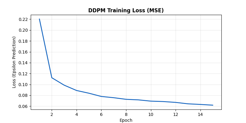
MSE loss over 15 epochs. Loss dropped from 0.2203 to 0.0619.
Why Uniform Timestep Sampling Matters
Since $t$ is sampled uniformly from $[0, T]$, the network must learn to denoise at every corruption level -- from near-clean images at $t \approx 10$ to pure noise at $t \approx 1000$. This is a harder objective than it sounds. At $t=10$, the image is almost pristine and the noise signal is tiny -- the network needs to detect and remove very faint perturbations. At $t=950$, the original image is almost entirely destroyed, and the network must hallucinate plausible structure from statistical hints. The uniform sampling forces a single 324K-parameter UNet to master both extremes and everything in between.
Generation: The Denoising Trajectory
To generate, we start from pure Gaussian noise $\mathcal{N}(0, \mathbf{I})$ and run the reverse process: at each step from $t=1000$ down to $t=0$, the network predicts the noise, we subtract a scaled fraction, and inject a small amount of fresh noise. The injected noise (sometimes called Langevin noise) is critical -- without it, all samples would collapse toward the same mean prediction, destroying diversity.
The trajectory reveals a clear phase structure. From $T=1000$ to roughly $T=600$, the image is indistinguishable from static -- no human could guess what digit is coming. Between $T=600$ and $T=400$, a vague blob begins to coalesce, narrowing down the class of possible digits. From $T=400$ to $T=100$, the digit identity locks in and the stroke geometry sharpens. The final stretch from $T=100$ to $T=0$ is pure refinement: cleaning up edges, evening out ink density, and resolving fine serifs or curves.
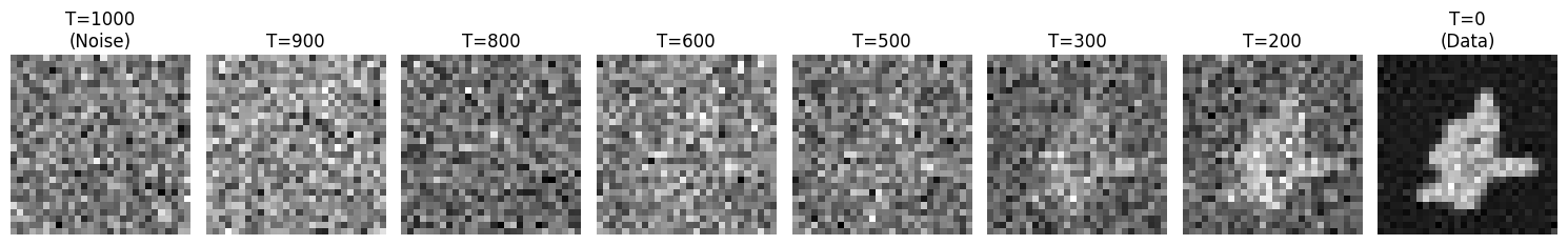
Reverse process from $T=1000$ to $T=0$. Digit shape stays ambiguous until roughly $T=400$, then fine details emerge.
The Final Generation Grid
Running the full 1,000-step reverse process on 32 independent noise seeds:
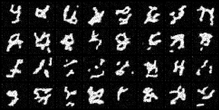
32 generated digits from independent noise seeds. None exist in the training set.
The outputs vary in slant, stroke width, and style -- the network learned the distribution, not a lookup table. Unlike an autoencoder, which compresses and reconstructs existing images, the diffusion model maps from a generic isotropic Gaussian prior to the full multi-modal data distribution. Each of the 32 samples above started from a different random seed and converged to a different digit with its own handwriting characteristics.
Why DDPMs Over GANs and VAEs
DDPMs solve a problem that GANs and VAEs struggled with: stable, high-fidelity generation from a simple Gaussian prior to a complex data distribution. GANs require a fragile adversarial equilibrium between generator and discriminator -- mode collapse, training instability, and hyperparameter sensitivity are constant risks. VAEs produce stable training but tend toward blurry outputs because they optimize a reconstruction loss that averages over the posterior.
DDPMs sidestep both issues. By decomposing the generation problem into 1,000 small denoising steps, each step only needs to make a minor correction. The network never has to learn a single giant mapping from noise to data. The training objective is a plain MSE loss -- no adversary, no KL divergence balancing act. The result is a model that trains stably and produces sharp, diverse outputs.
Conclusion
This was built entirely from scratch in PyTorch -- no external diffusion libraries, no pre-trained weights. A 324,705-parameter UNet, 15 epochs on MNIST, trained on Apple Silicon. The model goes from isotropic Gaussian static to recognizable handwritten digits through a 1,000-step reverse Markov chain, each step guided by a learned noise prediction.
The same core algorithm -- predict $\epsilon$, subtract, repeat -- scales from this 28x28 grayscale experiment all the way to the 1024x1024 text-conditioned generation in models like Stable Diffusion. The math does not change. The architecture gets bigger, the conditioning gets richer, but the fundamental loop is what we built here.