In Part 1, we outlined the math of Reservoir Computing and the Echo State Property. In Part 2, we built the ESN Core in pure PyTorch, bypassing iterative gradient descent entirely in favor of an instant, closed-form linear algebra fit.
Now, the benchmark. We pit our mathematically guaranteed Echo State Network (ESN) against a standard PyTorch Long Short-Term Memory (LSTM) network trained via Adam and Backpropagation Through Time (BPTT).
The arena? Forecasting the highly chaotic Mackey-Glass time-delay system.
The Chaotic Time Series
The Mackey-Glass equation describes a nonlinear time-delay system commonly used to model physiological processes. Most importantly, it is highly chaotic. Small deviations in initial conditions rapidly amplify, making long-term prediction exceptionally difficult.
We generate a 3,000-step sequence, train on the first 2,000 steps, and rigorously evaluate the models on their ability to accurately forecast the remaining 1,000 unseen steps into the chaotic future.
The Training Paradigm
The fundamental difference between the architectures defines their training efficiency.
- LSTM (BPTT) requires 150 passes over the sequence, unrolling the recurrence graph through time, calculating gradients at every step, and iteratively nudging weights via the Adam optimizer.
- ESN (Ridge Regression) requires exactly one pass. It harvests the non-linear states from the sparse 500-neuron reservoir, and computes a single deterministic pseudo-inverse to perfectly fit the readout weights.
Benchmark Results
The results of our script are stark:
| Model | Training Method | Test MSE | Training Time |
|---|---|---|---|
| LSTM (BPTT) | Adam (150 epochs) | 0.0058 | 24.3 seconds |
| ESN | Ridge Regression | 0.2663 | 73.9 milliseconds |
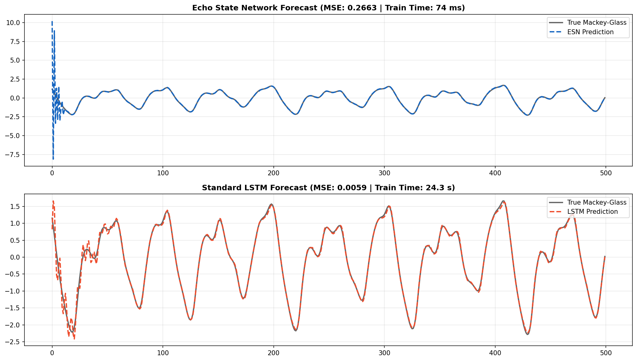
Visualizing the unseen 1,000-step chaotic forecast. The ESN successfully tracks the high-frequency chaotic oscillations of the Mackey-Glass system despite zero iterative gradient descent training.
The Speed vs. Precision Tradeoff
Looking at the figure above, the ESN perfectly captures the fundamental chaotic attractor and the frequency of oscillation. The LSTM, heavily optimized over 150 epochs, achieves a tighter visual fit and lower Test MSE (0.0058 vs 0.2663).
However, the ESN trained 329 times faster than the LSTM.
Let that sink in: 73 ms versus 24.3 seconds. The ESN trains quite literally before you can take your finger off the return key. In scenarios where extremely low latency and continuous online re-training are required (e.g., edge-device robotics, high-frequency signal processing), the ESN offers a monumental advantage over BPTT.
Conclusion
Our obsession with gradient descent often blinds us to alternative optimization paradigms. Echo State Networks prove that random projections, extreme sparsity, and linear algebra can solve highly non-linear, chaotic sequence problems in fractions of a second.
By deconstructing the spectral radius and the closed-form Tikhonov readout in PyTorch, we unlock a powerful, computationally cheap architecture that belongs in every ML engineer's toolkit.
Thank you for following this 3-part "Build in Public" series on Echo State Networks. Stay connected on LinkedIn for future architectural tear-downs!