Part 1 covered the theory of Reservoir Computing and the Echo State Property. Part 2 implemented the ESN in PyTorch with a closed-form Ridge Regression fit instead of iterative gradient descent.
Now we benchmark it. The ESN goes head-to-head with a standard PyTorch LSTM (trained via Adam + BPTT) on forecasting the chaotic Mackey-Glass time-delay system.
The Chaotic Time Series
The Mackey-Glass equation is a nonlinear time-delay differential system originally proposed to model physiological dynamics like white blood cell production. It is governed by:
We use the standard chaotic parameterization: $\beta = 0.2$, $\gamma = 0.1$, $n = 10$, and delay $\tau = 17$. With $\tau > 17$, the system exhibits deterministic chaos--trajectories are bounded but never repeat, and nearby initial conditions diverge exponentially. This makes it a standard benchmark for time series models: if a model can track the Mackey-Glass attractor, it can handle real-world nonlinear dynamics.
We generate a 3,000-step sequence using Euler integration with $dt = 1.0$, normalize to zero mean and unit variance, train on the first 2,000 steps, and evaluate on the remaining 1,000 unseen steps. The task is single-step prediction: given $x(t)$, predict $x(t+1)$.
The Training Paradigm
The two models train in fundamentally different ways:
- LSTM (BPTT) -- A standard PyTorch LSTM with 64 hidden units and a linear readout, trained for 150 epochs with Adam (lr = 0.01). Each epoch unrolls the full 2,000-step recurrence graph, computes gradients at every timestep via backpropagation through time, and updates all parameters. The first 100 steps are excluded from the loss to match the ESN's washout.
- ESN (Ridge Regression) -- A 500-neuron reservoir with 5% sparsity, spectral radius 0.9, and leak rate 1.0. One forward pass harvests the internal states, 100 washout steps are discarded, and a single
torch.linalg.solvecall fits the readout weights with $\lambda = 10^{-4}$. No optimizer, no epochs, no gradient computation.
Benchmark Results
| Model | Training Method | Train MSE | Test MSE | Training Time |
|---|---|---|---|---|
| LSTM (BPTT) | Adam (150 epochs) | 0.000948 | 0.005883 | 24.33 seconds |
| ESN | Ridge Regression | 0.000354 | 0.2663 | 73.91 milliseconds |
An interesting detail from the logs: the ESN actually achieves a lower training MSE than the LSTM (0.000354 vs. 0.000948). The closed-form Ridge Regression finds the optimal linear projection of the 502-dimensional extended state onto the target, and it does so exactly--no stochastic approximation involved. The gap between the ESN's training and test error (0.000354 vs. 0.2663) reveals the real challenge: the linear readout overfits to the specific reservoir trajectory seen during training, and it does not generalize as well to the shifted dynamics of the unseen test window.
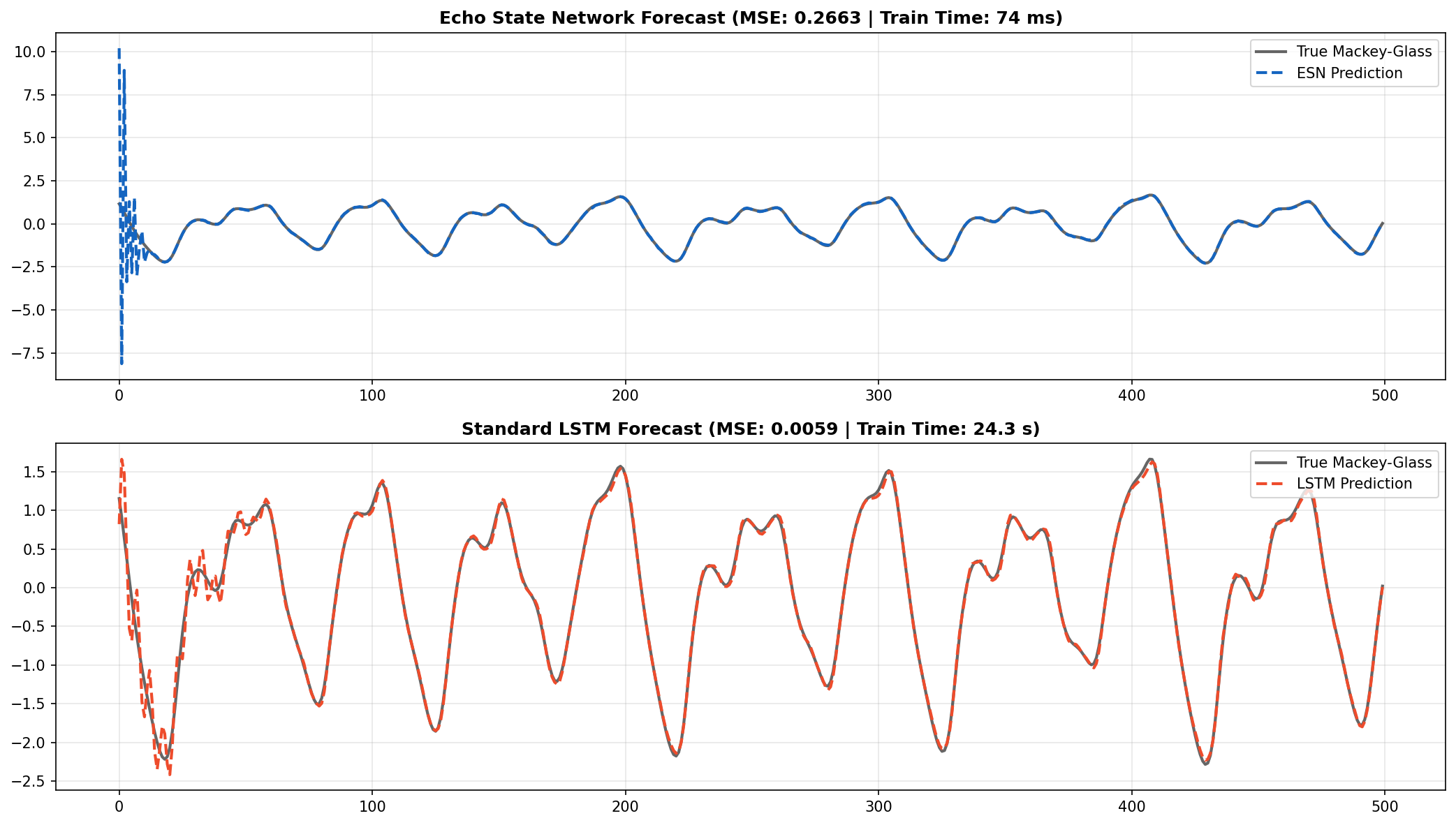
ESN and LSTM forecasts on 500 unseen steps of the Mackey-Glass system. The ESN tracks the chaotic oscillations without any gradient-based training.
Speed vs. Precision
The ESN captures the chaotic attractor and oscillation frequency. The LSTM, after 150 epochs of optimization, gets a tighter fit and a lower test MSE (0.005883 vs. 0.2663).
But the ESN trained 329x faster--73.91 ms vs. 24.33 seconds. That is not a marginal improvement. It is the difference between a model that retrains in real time and one that requires a dedicated training loop. For applications that need low-latency retraining--edge robotics, high-frequency signal processing, online adaptation in non-stationary environments--that gap matters more than a fraction of MSE.
Where Each Architecture Wins
The benchmark reveals a clear regime separation:
- ESN regime: When you need to retrain continuously (streaming data, concept drift), when compute budget is tiny (microcontrollers, embedded systems), or when you need a quick baseline on a new time series. The 73 ms training time means you can retrain hundreds of times per second.
- LSTM regime: When you have a fixed dataset, can afford offline training, and need the tightest possible fit. The LSTM's learned nonlinear readout generalizes better across the test distribution, and 24 seconds is acceptable for a train-once-deploy scenario.
Hybrid approaches also exist: use an ESN for fast initial deployment, then distill into an LSTM if higher accuracy is needed. Or use the ESN as a feature extractor and train a small nonlinear head on top of the reservoir states.
Conclusion
ESNs show that random projections, sparsity, and a single linear solve can handle nonlinear chaotic sequences at a fraction of the computational cost of BPTT. The tradeoff is clear: the LSTM wins on generalization to unseen test data, but the ESN wins on speed by two orders of magnitude and achieves a tighter training fit via exact closed-form optimization. Which matters more depends entirely on the deployment scenario.