Part 1 covered the minimax objective and the JSD connection. Part 2 built a Vanilla GAN and DCGAN in PyTorch. Now we train both on MNIST and see what actually happens.
Experimental Setup
Both architectures trained on a 5,000-image subset of MNIST for 50 epochs:
- Batch size: 64 (78 batches per epoch)
- Optimizer: Adam, $\text{lr} = 0.0002$, $\beta_1 = 0.5$, $\beta_2 = 0.999$
- Loss: BCELoss
- Noise: $z \in \mathbb{R}^{100}$ sampled from $\mathcal{N}(0, 1)$
- Data normalized to $[-1, 1]$ to match Tanh output
Parameter counts: the Vanilla GAN has 1,489,936 Generator and 533,505 Discriminator parameters. The DCGAN has a larger Generator (1,948,545 params) but a much smaller Discriminator (138,817 params) --- nearly 4$\times$ fewer than the Vanilla version.
Training Dynamics: Vanilla GAN
At epoch 1, the Generator loss is 0.7260 and the Discriminator loss is 1.3190. The Discriminator is still uncertain, and the Generator's random outputs happen to produce moderate loss thanks to the weight initialization.
Epochs 1--10 are rough. Generator loss swings between 0.73 and 1.30; Discriminator loss bounces from 1.14 to 1.37. This is typical early adversarial training --- both networks are reacting to each other's latest update, so the losses oscillate.
Things settle around epoch 20. Generator loss narrows to 1.1--1.3, Discriminator to 1.16--1.23. From epoch 25 onward, the Generator loss trends downward (from ~1.15 to 1.01) while the Discriminator loss drifts up toward 1.28 --- the Generator is slowly winning.
Final losses: $D_{\text{loss}} = 1.2590$, $G_{\text{loss}} = 1.0170$.
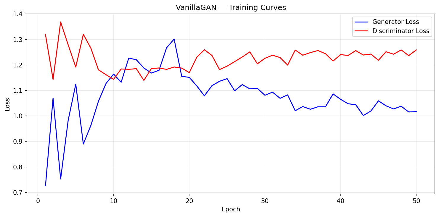
Vanilla GAN loss curves over 50 epochs. The oscillatory early dynamics settle into a slow Generator advantage by epoch 25.
Training Dynamics: DCGAN
The DCGAN starts in a very different place. At epoch 1, the Discriminator dominates: $D_{\text{loss}} = 0.4209$ vs. $G_{\text{loss}} = 2.8038$. The convolutional discriminator immediately learns to separate random feature maps from real digits.
Recovery is fast. By epoch 4, Generator loss drops to 0.9791. By epoch 10, both losses converge to the 1.05--1.10 range. From epoch 15 on, training is stable: $D_{\text{loss}}$ stays around 1.12--1.14, $G_{\text{loss}}$ near 1.05--1.09.
Final losses: $D_{\text{loss}} = 1.1260$, $G_{\text{loss}} = 1.0936$.
The smoother convergence comes directly from the convolutional structure. Both networks operate in a more constrained parameter space with built-in spatial priors, which cuts down on the oscillatory dynamics of fully-connected GANs.
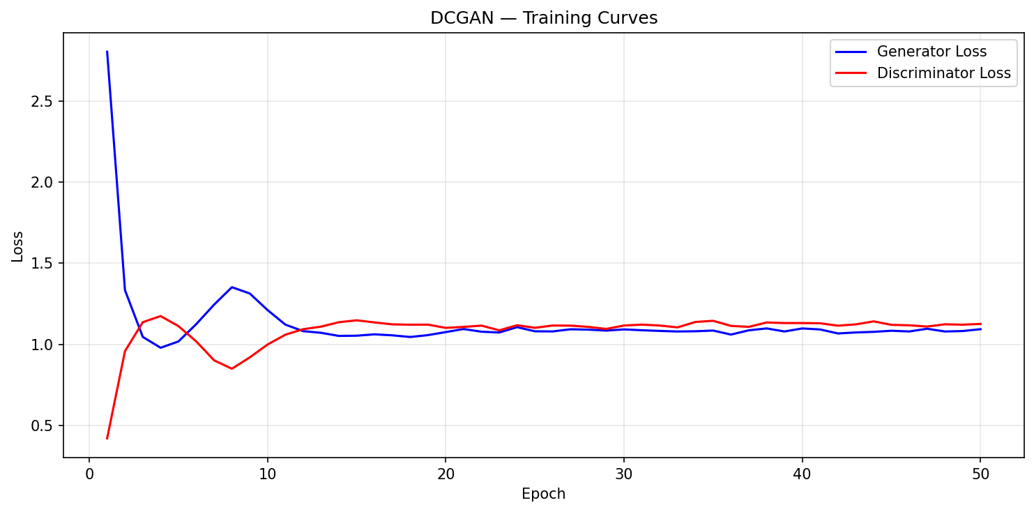
DCGAN loss curves over 50 epochs. After the initial Discriminator dominance (epoch 1), both losses converge quickly and stay stable.
Generated Sample Quality
Vanilla GAN
After 50 epochs, the Vanilla GAN produces recognizable digits --- 0s, 1s, 3s, 5s, 7s are identifiable across the grid. But the samples have visible artifacts:
- Speckling: Random bright pixels in the background. The fully-connected layers treat each pixel independently, so there is no spatial smoothness.
- Fuzzy edges: Strokes lack sharp boundaries.
- Uneven thickness: Stroke widths vary within a single digit.
The root cause is that the Generator predicts all 784 pixels independently --- there is nothing enforcing that adjacent pixels should be correlated.
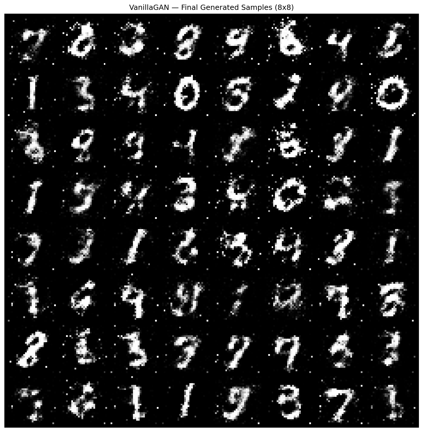
Vanilla GAN samples after 50 epochs. Digits are recognizable but noisy, with speckling artifacts and fuzzy stroke edges.
DCGAN
The DCGAN samples are noticeably sharper:
- Clean strokes with consistent thickness
- All 10 digit classes represented, with natural style variation
- Dark backgrounds with minimal noise
- Proper centering and proportions from the spatial awareness of transposed convolutions
The DCGAN gets better quality with a Discriminator that is 4$\times$ smaller (138K vs. 533K parameters). Convolutions provide enough inductive bias that the network needs far fewer parameters to learn the real-vs-fake boundary.
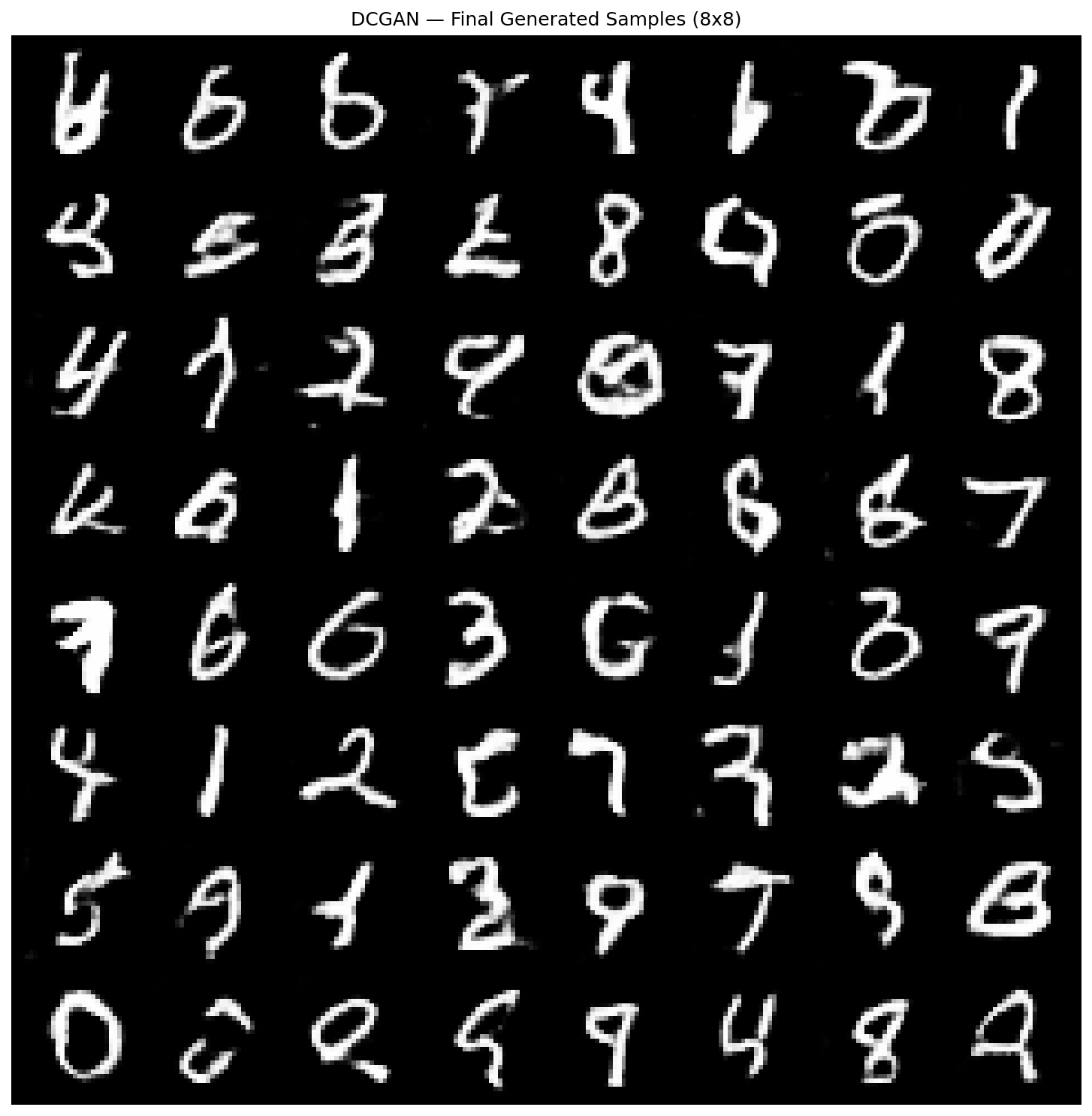
DCGAN samples after 50 epochs. Sharper strokes, cleaner backgrounds, and all 10 digit classes represented.
Mode Collapse Analysis
Neither model shows severe mode collapse --- both sample grids contain diverse digit classes. The Vanilla GAN does show mild mode preference, producing more 7s and 1s than 2s or 6s. The DCGAN's class distribution is more uniform.
Mode collapse happens when the Generator finds a small set of outputs that consistently fool the Discriminator, and the Discriminator cannot adapt quickly enough. The DCGAN's faster convergence gives less opportunity for this failure mode to take hold.
Connections to Other Generative Models
For context, here is how GANs compare to other generative frameworks:
- VAEs optimize a tractable ELBO and have stable training with a structured latent space, but tend to produce blurry samples.
- GANs produce sharper outputs via adversarial training, at the cost of training instability and no density estimate.
- Diffusion Models achieve state-of-the-art quality by iterative denoising, but need hundreds of forward passes at inference.
- Normalizing Flows give exact likelihoods through invertible transforms, but the bijectivity constraint limits architecture choices.
The adversarial training idea has leaked into all of these. Adversarial losses are commonly added to reconstruction objectives in hybrid models, and the discriminator concept evolved into critic networks (WGAN) and classifier-free guidance in diffusion models.
Conclusion
Across these three posts, we went from the minimax objective to trained models generating handwritten digits from 100-dimensional noise. The main takeaway: architectural details like LeakyReLU, BatchNorm placement, and weight initialization are not optional polish --- they determine whether training converges or collapses. And the jump from fully-connected to convolutional structure is substantial, producing cleaner outputs with fewer discriminator parameters.