Deconstructing Predictive Coding Networks: Part 3 - Benchmark Showdown

Introduction

Part 1 covered the theory. Part 2 built the PyTorch implementation. Now the question: how does a PCN actually perform against standard backpropagation?

We benchmark identical architectures -- one trained with backprop, one with local energy minimization -- on nonlinear regression and MNIST classification.

Experiment 1: Non-Linear Regression

We fit a noisy sine wave using both a standard MLP and a PCN, each with architecture 1 -> 32 -> 32 -> 1. The training data consisted of 1,000 points sampled uniformly from $[0, 4\pi]$ with Gaussian noise ($\sigma = 0.1$) added to the true sine values, trained in mini-batches of 32 over 50 epochs. The MLP used Adam (lr = 0.01) with standard backprop. The PCN ran 20 inference steps per sample (inference lr = 0.05) before applying the local Hebbian weight update (weight lr = 0.005). Both networks used Tanh activations.

Training Loss Comparison: Standard MLP vs PCN on nonlinear sine wave regression.

MLP vs PCN training loss on sine wave regression. The MLP converges faster with less noise.

Results

Both networks learned the sine function, but the dynamics differed:

MLP: Converged quickly to low MSE. Backprop has access to exact global gradients, so there is no ambiguity in the weight update direction.
PCN: Approximated the sine wave but with a noisier training curve. The noise comes from the inference phase: if latent nodes do not fully minimize their local prediction errors before the weight update, the subsequent gradient is misaligned. Inference learning rate tuning is critical. We also ran 30 inference steps at evaluation time (compared to 20 during training) to give the latent states more time to settle, which noticeably improved prediction quality on held-out regions of the sine curve.

Despite the noisier trajectory, the PCN's final regression fit was visually comparable to the MLP's. The key takeaway is not that local learning matches backprop on a smooth 1-D function -- it is that the PCN converged at all without any global gradient signal. Every weight update was computed from purely local variables: the pre-synaptic activation and the post-synaptic prediction error at each layer.

Experiment 2: Image Classification (MNIST)

Architecture: 784 -> 128 -> 10, classifying a 5,000-image subset of MNIST digits in batches of 64 over 10 epochs. The MLP used Adam (lr = 0.001) with cross-entropy loss. The PCN used 50 inference steps per batch (inference lr = 0.1, weight lr = 0.005) with supervised label clamping -- the top layer was fixed to the one-hot encoded target during the inference walk.

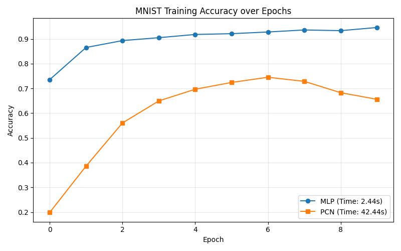
Test Accuracy Comparison: Standard MLP vs PCN on MNIST image classification.

MLP vs PCN test accuracy on MNIST. The MLP reaches >94%; the PCN climbs to 72% using only local learning.

This is where the PCN's generative nature creates specific challenges:

MLP: Hit >94% test accuracy within 10 epochs.
PCN: With ReLU activations, negative latent states got zero-gradient during inference, flatlining accuracy at 10% (random chance). Switching to Tanh and increasing inference steps to $T=50$ brought the PCN to 72% accuracy.

The key result: the PCN classified handwritten digits with zero global loss propagation, learning purely from local prediction errors at each layer.

Why PCNs Matter

Backprop wins on speed, accuracy, and stability. So why bother?

1. Algorithmic Biology: PCNs demonstrate that non-linear feature clustering (MNIST classification) can emerge from entirely local update rules. No global supervisor required.

2. Neuromorphic Hardware: Current GPU architectures are optimized for the backward pass -- global matrix multiplications and synchronous memory access. PCNs need none of that. Their local weight updates map directly onto neuromorphic chips (IBM NorthPole, analog crossbar arrays), where variable-resistance synapses update in place. Each synapse only needs access to its own pre- and post-synaptic signals -- no bus carrying a global error vector back through the network. This maps naturally to massively parallel analog hardware where millions of synapses can update simultaneously without waiting for a sequential backward pass.

3. Generative by Default: PCNs predict each layer's state from above, making them inherently bidirectional. A trained PCN can run in reverse -- fix a label at the top layer and let the inference walk relax downward to generate plausible inputs. This is not a retrofitted trick; it falls directly out of the top-down generative architecture. The same weights that learn to classify can also hallucinate, making PCNs a natural fit for tasks that require both discrimination and generation.