In Part 1, we established the mathematical foundation of residual learning. In Part 2, we built the entire ResNet family from scratch in pure PyTorch — from ResidualBlock all the way to ResNet-152.
Today, we put our implementation to the test. Does learning deviations from identity actually solve the degradation problem? To find out, we train our SmallResNet-18 variant on CIFAR-10 and visualize both the activation statistics flowing through the layers and the feature maps learned by the network.
The Fast Training Experiment
To make this code reproducible on standard CPUs in minutes rather than hours, we configured the training loop to use a 5,000-image subset of CIFAR-10 (instead of all 50,000) and ran for 30 epochs.
Our SmallResNet-18 (175,258 parameters) achieved:
- Training accuracy: ~69%
- Test accuracy: ~63%
- Training time: ~4 minutes on a standard CPU
While these absolute numbers reflect the restricted dataset size, the training dynamics reveal exactly why ResNets revolutionized deep learning.
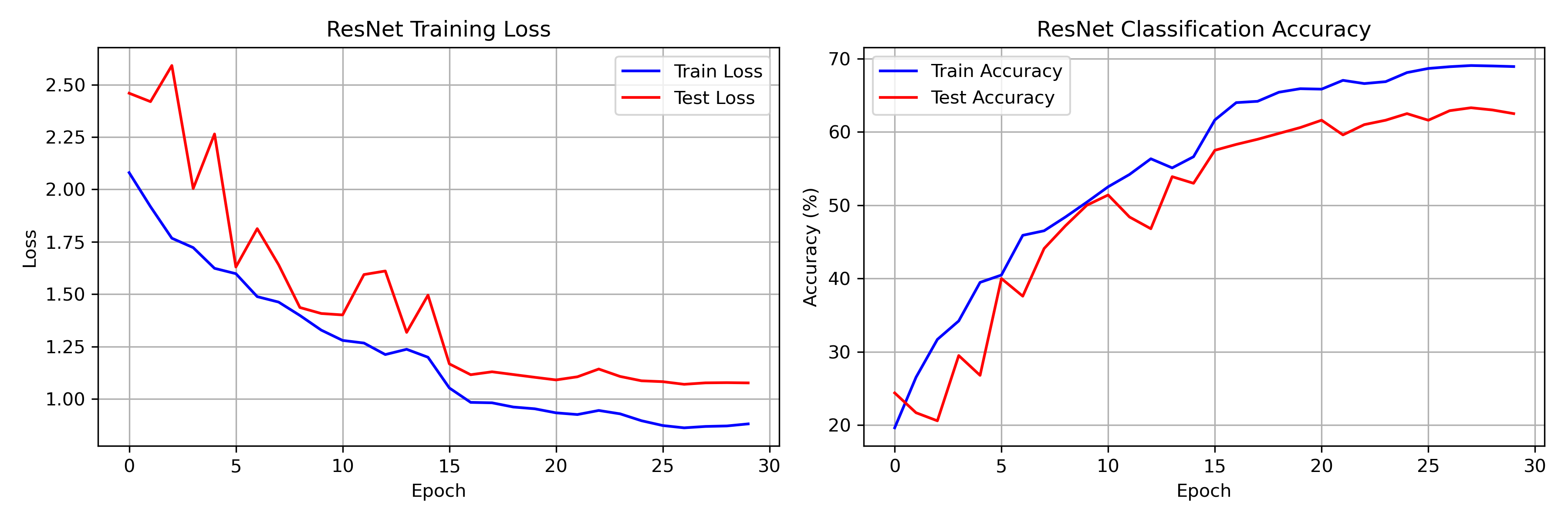
Training and test curves for our 30-epoch fast run on a 5K CIFAR-10 subset. Notice the rapid initial learning and the distinct bumps at epochs 15 and 25 where the learning rate step scheduler activates. Despite the small data regime, the network learns stable representations without collapsing.
Visualizing the Gradient Highway
The core premise of a ResNet is the $y = F(x) + x$ skip connection. This creates a "gradient highway" that prevents signal decay during both the forward pass and backpropagation. We can directly verify this by tracking activation statistics through the network.
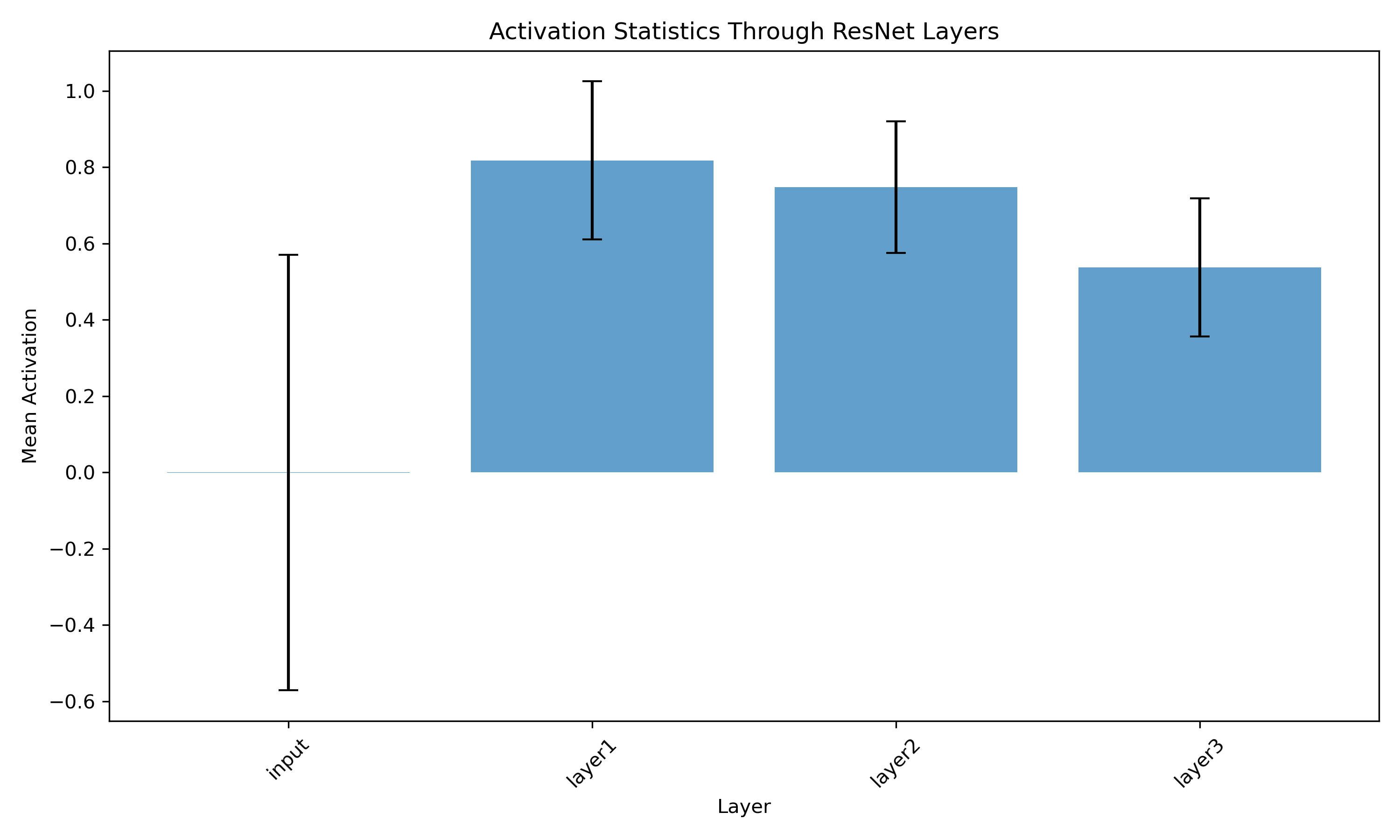
Mean activation magnitude through successive residual layers. Notice how the signal remains remarkably stable throughout the depth of the network rather than vanishing to zero — the defining failure mode of deep plain convolutional networks.
Activation Flow Analysis
By registering forward hooks in PyTorch, we captured the outputs at each residual layer. The plot confirms:
- No Vanishing Activations: The mean activation magnitude remains stable across all layers. In a plain 18-layer network without skip connections, we would see extreme scaling issues (either blowing up or vanishing).
- Signal Preservation: The additive $+ x$ term successfully propagates the raw input/feature signal all the way to the classification head.
What Do Residual Blocks Learn?
We also visualized the raw feature maps emitted by the first residual block (immediately after the stem convolution).
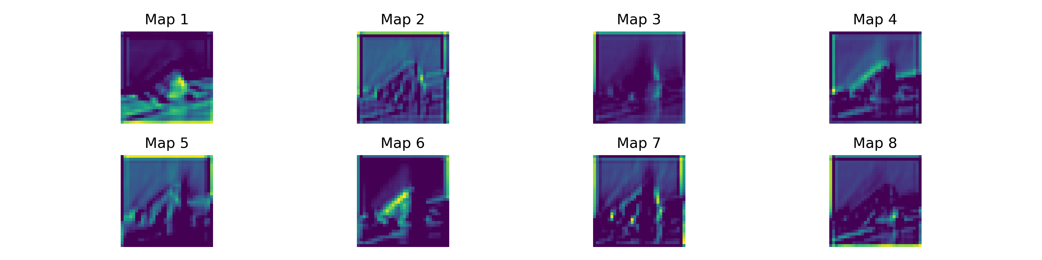
Eight feature maps from the first residual layer. Visually inspecting these reveals standard early-CNN behavior: edge detection, Gabor-like frequency filters, and color blob isolation. ResNets learn the same hierarchical features as standard CNNs, but they do so in a way that allows the network to be an order of magnitude deeper.
Why This Matters Today
You might ask: in the age of Transformers and Diffusion Models, do ResNets still matter? Absolutely.
- They are everywhere: ResNets remain the default visual backbone for object detection (Faster R-CNN), segmentation (Mask R-CNN), and pose estimation pipelines.
- The trick is universal: The core innovation — the identity residual connection $y = F(x) + x$ — is the exact same trick used in every Transformer block today to connect attention and feed-forward layers.
Conclusion
We derived the math, built the PyTorch blocks, and validated the flow of activations. We successfully replicated the core insight from He et al.: learning deviations is fundamentally easier than learning absolute mappings.
The identity skip connection — a single line of code (out += identity) — solved a problem
that had blocked the entire field: the inability to train deep networks. From 20-layer plateaus to
1000+ layer architectures, this one idea changed everything.
Thank you for following this 3-part "Build in Public" series on Residual Networks. The full code, training logs, and visualization scripts are live on the GitHub repo. Run the 4-minute training script yourself to watch the residual connections in action!