Part 1 was the math. Part 2 was the PyTorch implementation. Now we run the thing and see whether residual connections actually do what the theory promises -- stable gradient flow through deep networks, no degradation.
We train our SmallResNet-18 on a CIFAR-10 subset and look at training curves, activation magnitudes per layer, and learned feature maps.
The Fast Training Experiment
To keep this reproducible on a laptop CPU, we used a 5,000-image subset of CIFAR-10 (10% of the full training set) and trained for 30 epochs. Total wall time: about 4 minutes.
Our SmallResNet-18 has 175,258 parameters. Final numbers from the training log:
- Final training loss: 0.8805 (down from 2.0799 at epoch 1)
- Final training accuracy: 68.92%
- Best test accuracy: 63.30% (epoch 28)
- Final test accuracy: 62.50%
These numbers are capped by the tiny dataset, not the architecture. What matters more is the shape of the training dynamics.
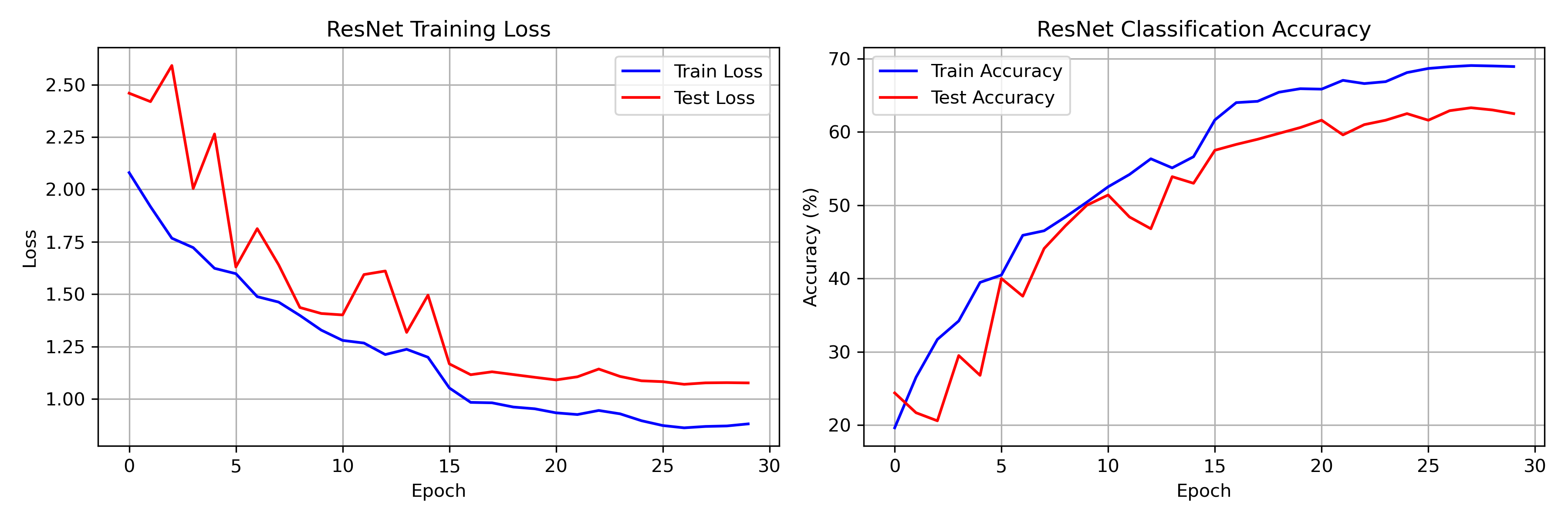
Loss and accuracy over 30 epochs on a 5K CIFAR-10 subset. The LR drops at epochs 15 and 25 produce visible jumps -- training loss falls from 1.20 to 1.05 after the first drop, and from 0.90 to 0.87 after the second.
Visualizing the Gradient Highway
The whole point of $y = F(x) + x$ is that the identity path keeps signal alive through depth. We can check this directly by recording activation magnitudes at each residual layer during a forward pass.
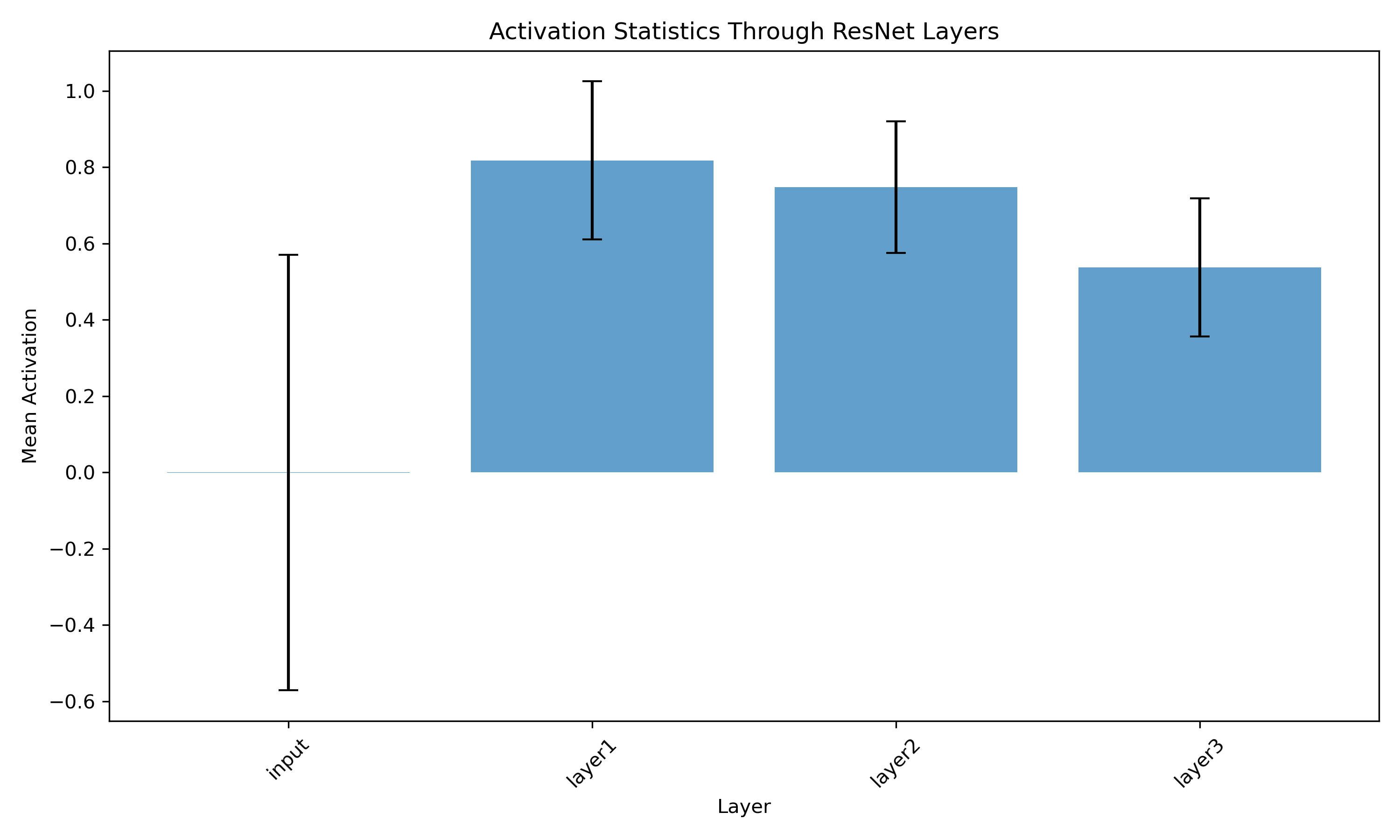
Mean activation magnitude across residual layers. Signal stays stable through the full depth of the network -- no vanishing, no explosion.
Activation Flow Analysis
We registered forward hooks on layer1, layer2, and
layer3 to capture output tensors. Two things stand out:
- No vanishing activations: Mean activation magnitude holds steady across all layers. A plain 18-layer network without skip connections would show either decay toward zero or blowup -- not this flat profile.
- Signal preservation: The $+ x$ term carries the input signal all the way to the classification head.
What Do Residual Blocks Learn?
We visualized the feature maps from the first residual block, right after the stem convolution.
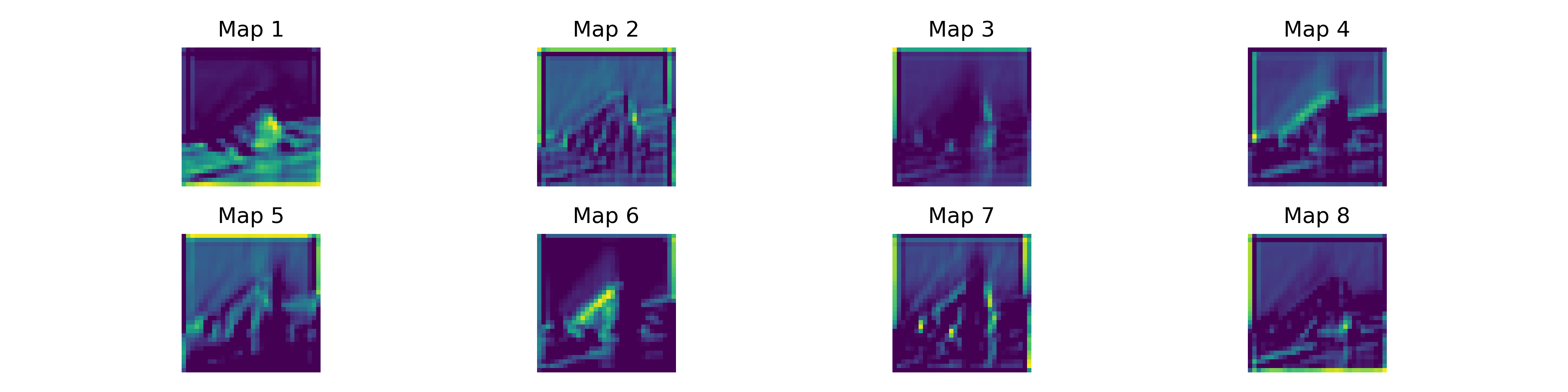
Eight feature maps from layer 1. Typical early-CNN patterns: edges, Gabor-like filters, color blobs.
These are the same types of features you see in any trained CNN. The difference is that ResNets can learn them reliably even when the network is an order of magnitude deeper.
Why This Matters Today
ResNets are from 2015, but the skip connection idea is everywhere now:
- Vision backbones: ResNets are still the default feature extractor in Faster R-CNN, Mask R-CNN, and most pose estimation pipelines.
- Transformers: Every Transformer block uses $y = F(x) + x$ to connect attention and feed-forward sublayers. Same residual connection, different $F$.
Conclusion
Across this series we went from the degradation problem to a working, trained ResNet. The activation plots confirm the theory: skip connections keep gradients and activations stable through depth. The core insight from He et al. -- learn deviations from identity, not absolute mappings -- turns out to be one of the most reusable ideas in deep learning.
Full code, training logs, and visualization scripts are on the GitHub repo. The training script runs in about 4 minutes on CPU.