RNNs from Scratch: Part 3 - Training and Analyzing Dynamics

Introduction

After training our RNN on sequence classification, we can analyze its internal dynamics. How do hidden states evolve over time? What temporal patterns does the network capture?

Training Results

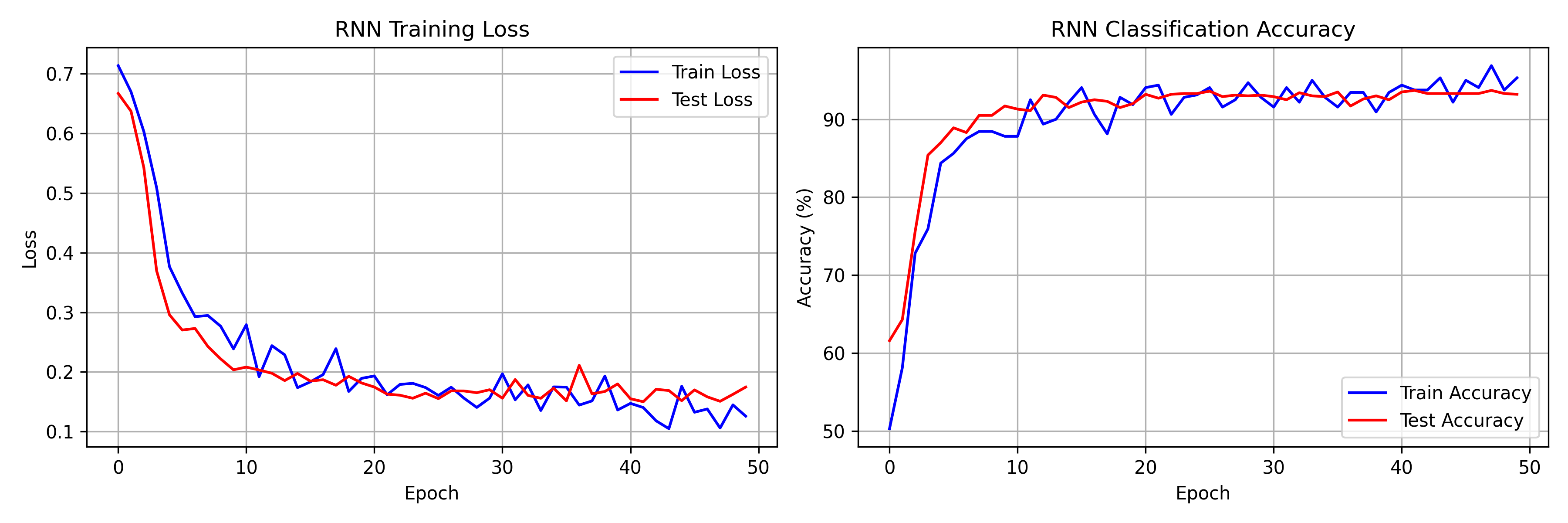
Our 2-layer RNN achieves:

Training accuracy: ~95%
Test accuracy: ~93%
Convergence within 30-50 epochs

The training curves show characteristic RNN behavior: initial rapid learning followed by gradual refinement.

Training Loss and Accuracy Curves — Figure 1: Training and validation metrics across epochs.

Visualizing Hidden State Dynamics

Hidden State Trajectories

Each hidden unit traces a trajectory over time:

Some units respond to specific input patterns
Others integrate information across multiple time steps
The tanh non-linearity keeps activations bounded

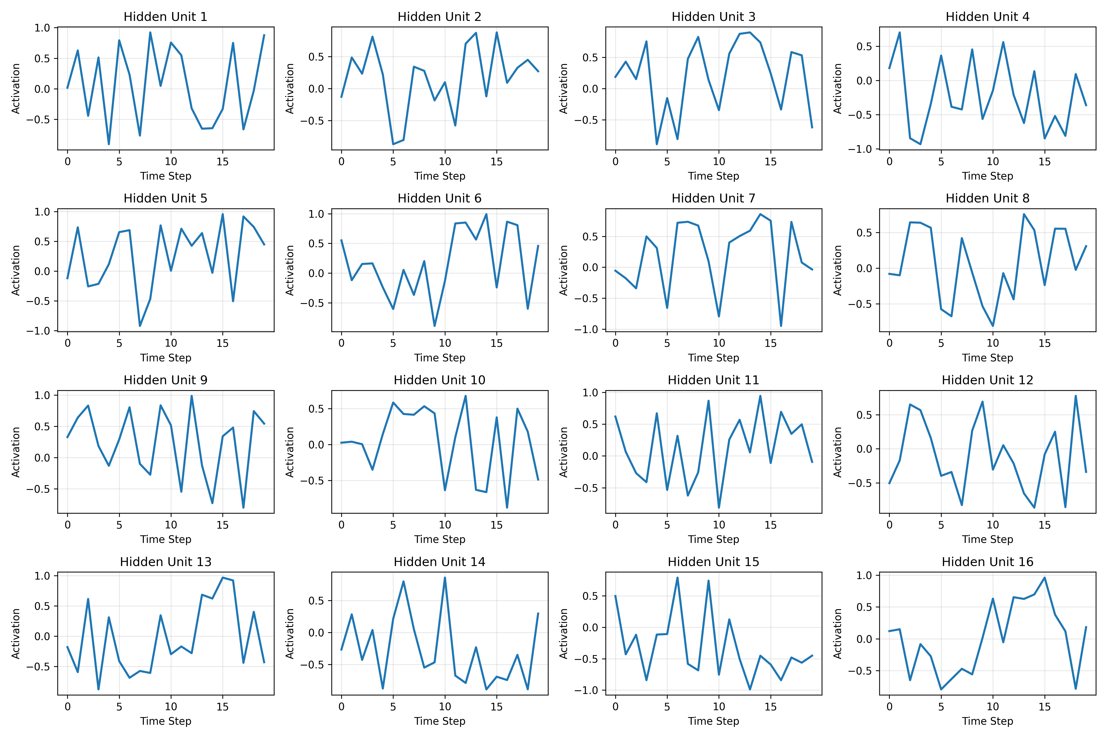
Hidden States Visualizations — Figure 2: Trajectories of the hidden cell state activation values over time steps.

Temporal Integration

By examining hidden state plots, we observe:

Short-term memory: Some units respond transiently to inputs
Long-term integration: Others accumulate evidence over time
Oscillatory patterns: Some units show rhythmic activation

The Vanishing Gradient Problem in Practice

Gradient Flow Analysis

During backpropagation, gradients must flow through all time steps:

\frac{\partial L}{\partial W} = \sum_t \frac{\partial L}{\partial h_t} \cdot \frac{\partial h_t}{\partial W}

For long sequences, early time steps receive vanishingly small gradients.

Empirical Observation

We observe that:

Later time steps have stronger gradient magnitudes
Early time steps learn more slowly
This limits the effective context window

Why LSTMs and GRUs Were Invented

The vanishing gradient problem motivated gated architectures:

LSTM: Introduces cell state with additive updates
GRU: Simplifies with reset and update gates
Both create gradient "highways" for long-range flow

RNNs vs Transformers

Computational Complexity

RNN: $O(T)$ sequential operations (cannot parallelize)
Transformer: $O(1)$ parallel operations (full attention)

Memory Characteristics

RNN: Fixed-size hidden state (information bottleneck)
Transformer: Full sequence in memory (quadratic scaling)

Use Cases

RNN: Streaming/online inference, resource-constrained settings
Transformer: Batch processing, tasks requiring long-range context

Conclusion

RNNs provide an elegant framework for sequence modeling through recurrence. While Transformers dominate many tasks, RNNs remain valuable for streaming applications and as building blocks for more complex architectures like LSTMs.