RNNs from Scratch: Part 3 - Training and Analyzing Dynamics

Introduction

With the RNN implemented, we train it on a synthetic sequence classification task and dig into the results. This post covers the training numbers, hidden state visualizations, and a practical look at where vanilla RNNs break down.

Training Results

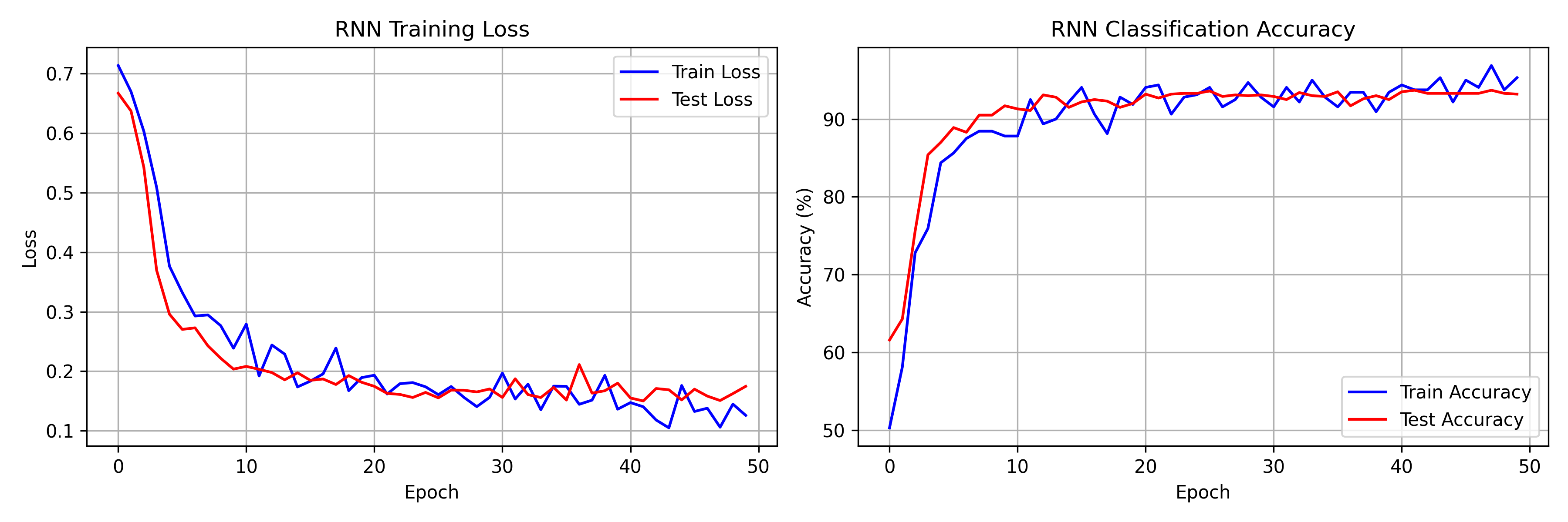
The model has 13,314 parameters and was trained for 50 epochs on CPU. Final numbers from the run:

Training accuracy: 95.31% (loss: 0.1258)
Test accuracy: 93.20% (loss: 0.1746)
Best test accuracy: 93.70% at epoch 42

Most of the learning happens in the first 10 epochs, with train accuracy jumping from 50.31% to 87.81% and test loss dropping from 0.6670 to 0.2036. After that, gains are incremental -- the model plateaus around 93% test accuracy by epoch 20 and fluctuates there for the remaining 30 epochs. The learning rate scheduler halves the rate at epoch 20, which briefly tightens the loss curves, but the network is already near its capacity on this task.

Training Loss and Accuracy Curves — Loss and accuracy over 50 epochs. The sharp drop in loss during epochs 1-10 gives way to noisy plateaus.

Visualizing Hidden State Dynamics

Hidden State Trajectories

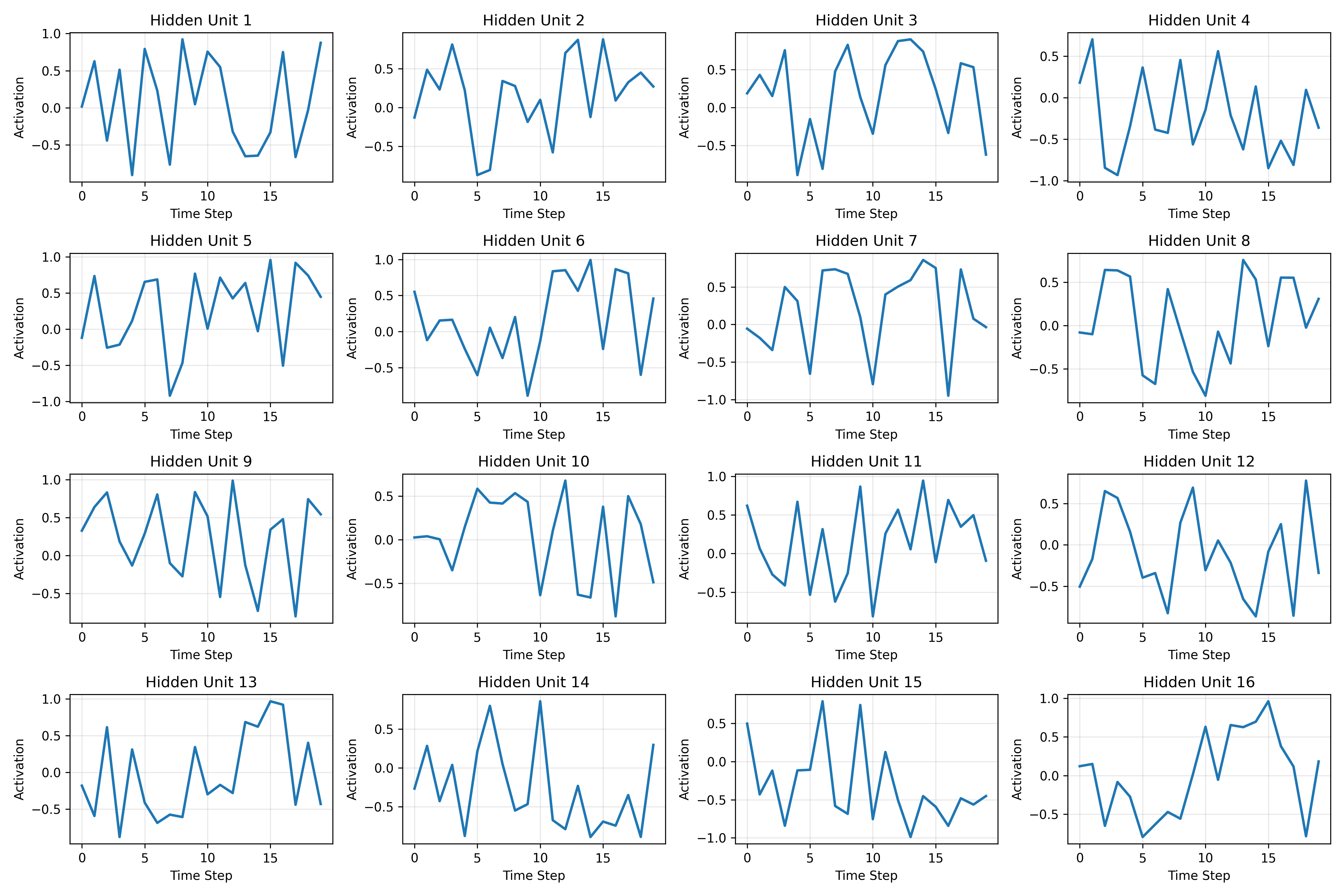
Plotting individual hidden units across time steps reveals different roles. Some units spike in response to specific input patterns and reset quickly. Others ramp up gradually, integrating information over multiple steps. The tanh squashing keeps all activations in $[-1, 1]$, which you can see clearly in the plots below.

Hidden States Visualizations — Hidden unit activations over time steps for a sample input sequence.

Temporal Integration

Three broad behaviors show up across the 64 hidden units:

Transient response -- units that fire briefly at specific inputs then decay back toward zero within a few steps
Accumulation -- units that build up a running signal over multiple steps, effectively tracking a cumulative statistic of the input
Oscillation -- units that alternate between positive and negative activation, potentially encoding periodic patterns

The classification task requires computing a global mean, so the accumulator units are doing most of the heavy lifting. They approximate a running average, and the final-step readout extracts the sign of that average for the binary label. The transient and oscillatory units likely encode finer-grained patterns that help with boundary cases.

The Vanishing Gradient Problem in Practice

Gradient Flow Analysis

The total gradient with respect to the weights sums contributions from every time step:

\frac{\partial L}{\partial W} = \sum_t \frac{\partial L}{\partial h_t} \cdot \frac{\partial h_t}{\partial W}

In practice, the contributions from early time steps are orders of magnitude smaller than those from later steps. Each backward step multiplies by $W_{hh}^T \cdot \text{diag}(1 - \tanh^2(\cdot))$, and with tanh derivatives bounded between 0 and 1, the product shrinks rapidly.

What This Looks Like in Practice

The consequence is straightforward:

Gradient magnitudes are much larger at later time steps
The network barely updates its weights based on early inputs
The effective context window is shorter than the actual sequence length

For our 20-step sequences this is manageable -- the network still reaches 93.7% test accuracy. But scale up to sequences of length 100 or 500, and the model would struggle to learn dependencies that span the full input. The training loss would stall at a higher value, and early-sequence information would be effectively invisible to the optimizer.

Why LSTMs and GRUs Were Invented

The vanishing gradient problem motivated gated architectures:

LSTM: Introduces cell state with additive updates
GRU: Simplifies with reset and update gates
Both create gradient "highways" for long-range flow

RNNs vs Transformers

Computational Complexity

RNN: $O(T)$ sequential operations (cannot parallelize)
Transformer: $O(1)$ parallel operations (full attention)

Memory Characteristics

RNN: Fixed-size hidden state (information bottleneck)
Transformer: Full sequence in memory (quadratic scaling)

Use Cases

RNN: Streaming/online inference, resource-constrained settings
Transformer: Batch processing, tasks requiring long-range context

Wrapping Up

Our 13K-parameter RNN hits 93.7% test accuracy on this synthetic task, which is decent but clearly limited. The vanishing gradient problem is not just theoretical -- it shows up directly in the gradient magnitudes and in the network's inability to use early sequence information. LSTMs and GRUs were designed specifically to fix this, and Transformers sidestep it entirely with attention. Still, RNNs are worth understanding: they are simple, memory-efficient for streaming inference, and the foundation for everything that came after.